Introduction/Background
There are numerous amounts of research and evidence revealing that stock prices can be predicted and are affected by various aspects of daily life, which can ultimately help an investor. One such aspect of daily life is news, where general news occurring around the world and in the country can affect the movement of certain stocks directly and indirectly. However, the bulk of research in this field focuses on financial news, rather than news as a whole. With this in mind, our team set out to analyze the immediate change of stock prices as a reaction to general news stories. We chose to apply our models to Apple stock (AAPL) for this project because it represents a fairly stable stock and is heavily traded.
Problem Definition
This machine learning project is centered around analyzing news stories to predict the movement of Apple (AAPL) stock prices in the market. Research has shown that adding in predictors such as news stories and social media posts (ex: Twitter) makes significant improvements to the quality of stock price predictions (Vanstone et al., 2019). As mentioned, for this project, we looked specifically at AAPL due to its relative stability and heavy trading. Instead of purely looking at financial news or Apple-related news, our models utilized general news as a whole. We also had some models that included the Dow Jones Industrial Average information as a market index that captures the general market trend to see if combining general news with this financial data would provide a better prediction of prices. Furthermore, rather than simply predicting the rise and fall of AAPL (information which could help an investor decide whether or not to buy or sell shares), our models were designed to predict the exact prices (which would reveal more information to an investor compared to a prediction of only rise or fall). Ultimately, we sought to create models that would accurately predict the prices of AAPL which could be used as a tool for people and companies to aid them in their investment decisions.
Data Collection
We obtained our news article data from the NYT Developer API, taking the NYT archive data from January 2016 to
December 2020. By feeding the month and year to the API, we get JSON with an array of all articles from that
particular month. Rather than the full raw text of all the articles, we receive the metadata from these articles
such as headlines, abstract, and keywords. Thus, the NYT data was already relatively clean and extensive data
cleaning wasn’t needed. It was helpful to use the cleaned data rather than raw text from all the articles to avoid
storage and computing issues in our model. To obtain AAPL data, we used the yfinance library to access historical
financial AAPL stock data from Yahoo Finance from December 2015 to January 2021 (we added these two extra months to
account for price changes from January 2016 to December 2020). Though this data was also relatively clean, we still
had to perform some data cleaning and preprocessing before our data was ready. For example, we added extra features
to the Apple data that were not present in Yfinance like the percent change for a day. We also removed the news
article data from days the stock market was not open, including weekends and holidays, to ensure our model was using
the appropriate data.
The content of interest in the NYT news articles was the abstract. We decided to use BERT because “it’s conceptually
simple” and “obtained new state of the art results on … NLP tasks” (Devlin et al., 2019). In order to semantically
and contextually represent the abstract using BERT, it underwent some pre-processing. The given abstract was treated
as a single segment of data. After adding the classifier and separator tokens, the abstract was tokenized using
built-in tensorflow extensions for BERT. Tokenization involves converting all words into BERT tokens, and split up
any OOV (Out-of-Vocabulary) words into smaller tokens, prefixes, and suffixes. After tokenizing the data, it was
converted to indices to represent each token as an entry in BERT vocabulary, which is the reference index for BERT
to get the unique word embedding for the given vocabulary word.
Methods
By manipulating word and document embeddings generated by BERT for each news story abstract for a single day, a 768
dimension vector can be obtained, which is referred to as the “daily embedding” for the given day. The daily
embedding encapsulates the information from news stories on all given days into a R768 space. However, when dealing
with over 69000 new stories from several years, 768 features impose a great toll on computing power and memory at
disposal. As a result, the daily embeddings need to go through data reduction before inferences can be drawn from
them.
Accounting for 95% variance for features of all 69404 news stories in the dataset yields a staggering 83%
compression in space occupied by reducing the 768 dimensions to just 131. We were also able to reduce the thousands
of news stories by averaging all the vectors for a specific day. This lets us move from 69,000 data points to 365.
Following dimensionality reduction, the evolution of content in news stories is compared to the evolution of the
market for AAPL to look for trends within. Since the content of news on different days as well as market behavior
trends are spread across timelines, one could use LSTM (Long Short Term Memory) models, which are known for their
efficiency in time series. By training and testing the LSTM networks, the general trend of AAPL could be predicted.
For the LSTM networks, we utilize three LSTM layers and two drop out layers, and use ReLU(Rectified Linear Unit) as
an
activation function. We split the data into training and testing data with 8:2 ratio and scaled it with
MinMaxScaler of sckit-learn package since each feature has a different range. Then we trained our models with epochs
of 20
and batch size of 32.
$$ x' = \frac{x - min(x)}{max(x) - min(x)} $$
[Equation 1: min-max scaler]
Results and Discussion
1. LSTM with BERT-transformed NYT article abstracts of the past 60 days.
1.a. Raw BERT-transformed NYT article abastracts
-
Train feature data size:
(819, 60, 768) -
Train label data size:
(819,)
_________________________________________________________________
Layer (type)                 Output Shape              Param #
=================================================================
lstm_75 (LSTM)               (None, 60, 10)            31160
_________________________________________________________________
dropout_75 (Dropout)         (None, 60, 10)            0
_________________________________________________________________
lstm_76 (LSTM)               (None, 60, 20)            2480
_________________________________________________________________
dropout_76 (Dropout)         (None, 60, 20)            0
_________________________________________________________________
lstm_77 (LSTM)               (None, 30)                6120
_________________________________________________________________
dropout_77 (Dropout)         (None, 30)                0
_________________________________________________________________
dense_25 (Dense)             (None, 1)                 31
=================================================================
Total params: 39,791
Trainable params: 39,791
Non-trainable params: 0
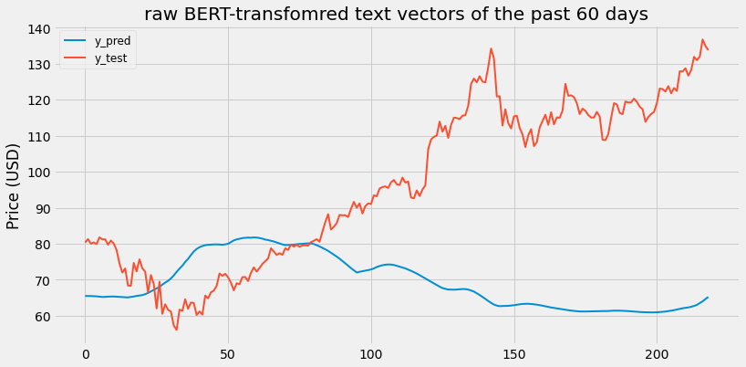
[Figure 1.1: LSTM with raw BERT-transformed NYT article abstracts of the past 60 days.]
Scaled RMSE: 0.48106433548771926
1.b. Dimension-reduced BERT-transformed NYT article abastracts
-
Train feature data size:
(817, 60, 127) -
Train label data size:
(817,)
_________________________________________________________________
Layer (type)                 Output Shape              Param #
=================================================================
lstm_69 (LSTM)               (None, 60, 10)            5520
_________________________________________________________________
dropout_69 (Dropout)         (None, 60, 10)            0
_________________________________________________________________
lstm_70 (LSTM)               (None, 60, 20)            2480
_________________________________________________________________
dropout_70 (Dropout)         (None, 60, 20)            0
_________________________________________________________________
lstm_71 (LSTM)               (None, 30)                6120
_________________________________________________________________
dropout_71 (Dropout)         (None, 30)                0
_________________________________________________________________
dense_23 (Dense)             (None, 1)                 31
=================================================================
Total params: 14,151
Trainable params: 14,151
Non-trainable params: 0
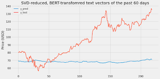
[Figure 1.2: LSTM with reduced BERT-transformed NYT article abstracts of the past 60 days.]
Scaled RMSE: 0.44102269317574305
From these two graphs, it’s clear that relying solely on text vectors to predict stock data leads to a bad result. This makes sense because additional features like stock prices and economic trends are required to get a more accurate prediction. The goal of our model is to see how text vectors integrate with other features so let’s check that out now.
2. LSTM with historical price of the past 60 days
2.a. LSTM with historical APPL price of the past 60 days
-
Train feature data size:
(820, 60, 3) -
Train label data size:
(820,)
Layer (type)                 Output Shape              Param #
=================================================================
lstm_6 (LSTM)                (None, 60, 10)            560
_________________________________________________________________
dropout_6 (Dropout)          (None, 60, 10)            0
_________________________________________________________________
lstm_7 (LSTM)                (None, 60, 20)            2480
_________________________________________________________________
dropout_7 (Dropout)          (None, 60, 20)            0
_________________________________________________________________
lstm_8 (LSTM)                (None, 30)                6120
_________________________________________________________________
dropout_8 (Dropout)          (None, 30)                0
_________________________________________________________________
dense_2 (Dense)              (None, 1)                 31
=================================================================
Total params: 9,191
Trainable params: 9,191
Non-trainable params: 0
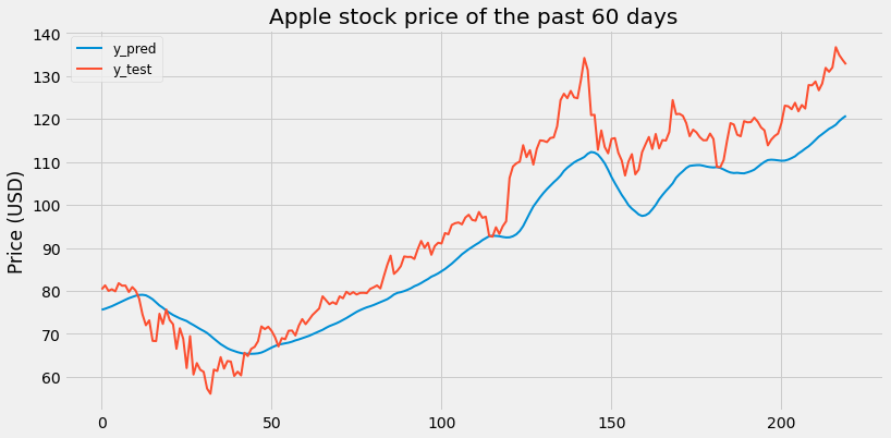
[Figure 2.1: LSTM with historical APPL price of the past 60 days]
Scaled RMSE: 0.11442445233714693
2.b. LSTM with historical APPL price and Dow Jones Index of the past 60 days
-
Train feature data size:
(820, 60, 4) -
Train label data size:
(820,)
_________________________________________________________________
Layer (type)                 Output Shape              Param #
=================================================================
lstm_24 (LSTM)               (None, 60, 10)            600
_________________________________________________________________
dropout_24 (Dropout)         (None, 60, 10)            0
_________________________________________________________________
lstm_25 (LSTM)               (None, 60, 20)            2480
_________________________________________________________________
dropout_25 (Dropout)         (None, 60, 20)            0
_________________________________________________________________
lstm_26 (LSTM)               (None, 30)                6120
_________________________________________________________________
dropout_26 (Dropout)         (None, 30)                0
_________________________________________________________________
dense_8 (Dense)              (None, 1)                 31
=================================================================
Total params: 9,231
Trainable params: 9,231
Non-trainable params: 0
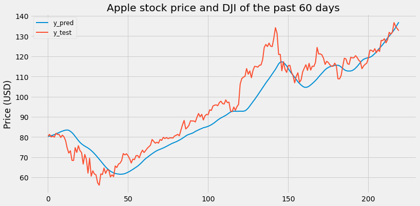
[Figure 2.2: LSTM with historical APPL price and Dow Jones Index of the past 60 days]
Scaled RMSE: 0.09475997994308416
Looking at previous Apple stock prices and the DJI leads to a good prediction of Apple stock. With a 91% accuracy, the predictions are already very satisfactory. Now let’s see whether incorporating text vectors improves the performance.
3. LSTM with historical price of the past 60 days and raw BERT-transformed NYT article abastracts.
3.a. LSTM with historical APPL price of the past 60 days and raw BERT-transformed NYT article abastracts.
-
Train feature data size:
(819, 60, 771) -
Train label data size:
(819,)
_________________________________________________________________
Layer (type)                 Output Shape              Param #
=================================================================
lstm_45 (LSTM)               (None, 60, 10)            31280
_________________________________________________________________
dropout_45 (Dropout)         (None, 60, 10)            0
_________________________________________________________________
lstm_46 (LSTM)               (None, 60, 20)            2480
_________________________________________________________________
dropout_46 (Dropout)         (None, 60, 20)            0
_________________________________________________________________
lstm_47 (LSTM)               (None, 30)                6120
_________________________________________________________________
dropout_47 (Dropout)         (None, 30)                0
_________________________________________________________________
dense_15 (Dense)             (None, 1)                 31
=================================================================
Total params: 39,911
Trainable params: 39,911
Non-trainable params: 0
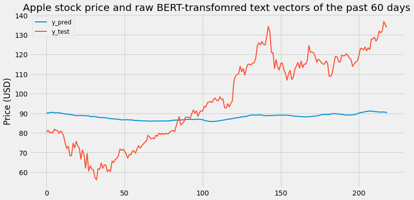
[Figure 3.1: LSTM with historical APPL price of the past 60 days and raw BERT-transformed NYT article abastracts]
Scaled RMSE: 0.3808984939602866
3.b. LSTM with historical APPL price and Dow Jones Index of the past 60 days and raw BERT-transformed NYT article abastracts.
-
Train feature data size:
(819, 60, 772) -
Train label data size:
(819,)
Layer (type)                 Output Shape              Param #
=================================================================
lstm_36 (LSTM)               (None, 60, 10)            31320
_________________________________________________________________
dropout_36 (Dropout)         (None, 60, 10)            0
_________________________________________________________________
lstm_37 (LSTM)               (None, 60, 20)            2480
_________________________________________________________________
dropout_37 (Dropout)         (None, 60, 20)            0
_________________________________________________________________
lstm_38 (LSTM)               (None, 30)                6120
_________________________________________________________________
dropout_38 (Dropout)         (None, 30)                0
_________________________________________________________________
dense_12 (Dense)             (None, 1)                 31
=================================================================
Total params: 39,951
Trainable params: 39,951
Non-trainable params: 0
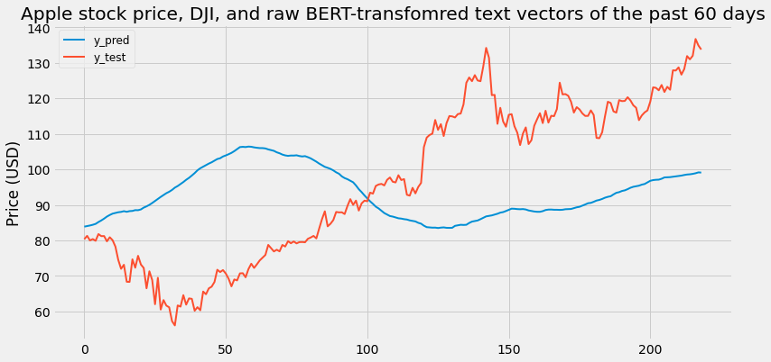
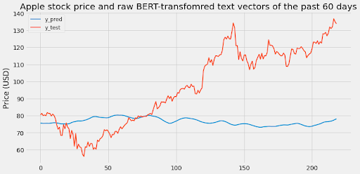
[Figure 3.2: LSTM with historical APPL price and Dow Jones Index of the past 60 days and raw BERT-transformed NYT article abastracts]
Scaled RMSE: 0.32082032270116007
Surprisingly, adding Daily Embeddings from BERT significantly decreases the performance of the model and rarely predicts correctly. One of the main reasons that happens is because 768 features is too high for a small dataset such as the one we are using. When using sparsely populated features, one needs significantly more data as compared to the features.
4. LSTM with historical price of the past 60 days and dimension-reduced BERT-transformed NYT article abastracts
4.a. LSTM with historical APPL price of the past 60 days and dimension-reduced BERT-transformed NYT article abastracts
-
Train feature data size:
(817, 60, 130) -
Train label data size:
(817,)
_________________________________________________________________
Layer (type)                 Output Shape              Param #
=================================================================
lstm_78 (LSTM)               (None, 60, 10)            5640
_________________________________________________________________
dropout_78 (Dropout)         (None, 60, 10)            0
_________________________________________________________________
lstm_79 (LSTM)               (None, 60, 20)            2480
_________________________________________________________________
dropout_79 (Dropout)         (None, 60, 20)            0
_________________________________________________________________
lstm_80 (LSTM)               (None, 30)                6120
_________________________________________________________________
dropout_80 (Dropout)         (None, 30)                0
_________________________________________________________________
dense_26 (Dense)             (None, 1)                 31
=================================================================
Total params: 14,271
Trainable params: 14,271
Non-trainable params: 0
[Figure 4.1: LSTM with historical APPL price of the past 60 days and dimension-reduced BERT-transformed NYT article abastracts]
Scaled RMSE: 0.2837049092158715
4.b. LSTM with historical APPL price and Dow Jones Index of the past 60 days and dimension-reduced BERT-transformed NYT article abastracts
-
Train feature data size:
(817, 60, 131) -
Train label data size:
(817,)
________________________________________________________________
Layer (type)                 Output Shape              Param #
=================================================================
lstm_81 (LSTM)               (None, 60, 10)            5680
_________________________________________________________________
dropout_81 (Dropout)         (None, 60, 10)            0
_________________________________________________________________
lstm_82 (LSTM)               (None, 60, 20)            2480
_________________________________________________________________
dropout_82 (Dropout)         (None, 60, 20)            0
_________________________________________________________________
lstm_83 (LSTM)               (None, 30)                6120
_________________________________________________________________
dropout_83 (Dropout)         (None, 30)                0
_________________________________________________________________
dense_27 (Dense)             (None, 1)                 31
=================================================================
Total params: 14,311
Trainable params: 14,311
Non-trainable params: 0
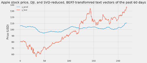
[Figure 4.2: LSTM with historical APPL price and Dow Jones Index of the past 60 days and dimension-reduced BERT-transformed NYT article abastracts]
Scaled RMSE: 0.2613873171396424
When reducing the data through SVD, the performance slightly increases since the number of features decrease. However, the existing 131 features are still sparsely populated and are therefore the leading cause of discrepancy in prediction. For 70000 data points, one should have much fewer features. For 131 dimensions to represent all features, one should have a lot more data points. Since the representation of text content has several features, it fails to help our model despite the state of the art accuracy in its niche field.
Conclusions
Though our models may not be the best predictors of Apple stock price to help investment decisions, there are
various factors that could have caused the error in predictions for our models. One of these factors is that
accurate stock price prediction models require a large amount of data, and a lot of different types of data. While
our models only took into account general news data, previous AAPL stock price data, and the Dow Jones Industrial
Average to capture market trends, there are a plethora of other aspects of daily life that largely influence stock
prices that we did not account for. Furthermore, news tends to be negative. Therefore, our predictions could have
been inaccurate due to the news being overly negative, which would cause the news sentiment data to inaccurately
represent the general sentiment of society.
Additionally, stock prediction is quite a difficult task. Various financial institutions expend billions of dollars
to improve their prediction algorithms because these prediction algorithms can be extremely useful when making
investment decisions. The COVID-19 pandemic also could have influenced our results, because this pandemic has
affected stock prices and has been the center of the news for the past year.
Ultimately, there are many options for us to fine-tune our models to improve stock price predictions. By doing more
research on the effects of news on stock prices, and to what degree news affects stock prices, our models may
improve. In addition, we could experiment with more stock data and note how prediction accuracy changes with
different levels of emphasis placed on specific features of stock data and news data in an attempt to improve
results. Overall, though our current models may not be a great resource to base investment decisions upon, our group
has deeply broadened our knowledge of machine learning models and their importance in the field of finance and
investing.
References
- Vanstone, B. J., Gepp, A., & Harris, G. (2019). Do news and sentiment play a role in stock price prediction? Applied Intelligence, 49(11), 3815–3820. https://doi.org/10.1007/s10489-019-01458-9
- Devlin, J., Chang, M.-W., Lee, K., & Toutanova, K. (2019, May 24). BERT: Pre-training of Deep Bidirectional Transformers for Language Understanding. arXiv.org. https://arxiv.org/abs/1810.04805?source=post_page.